Data Structures & Algorithms: Full lesson content. # Algorithms > Fundamental concepts of algorithms An algorithm is a step-by-step procedure or step-by-step instructions for solving a problem or completing a task. ## Characteristics of Good Algorithms [Section titled “Characteristics of Good Algorithms”](#characteristics-of-good-algorithms) 1. **Input** - Accepts zero or one or more inputs. 2. **Output** - Produces at least one output. 3. **Finiteness** - Terminates after a finite number of steps. 4. **Correctness** - Produces the correct output for all valid inputs. 5. **Definiteness** - Each step is clearly and unambiguously defined. 6. **Efficiency** - Uses minimal time (time complexity) and space (space complexity). # Big O Notation > Understanding algorithm complexity and performance analysis Big O notation is a way to describe how the running time or space requirements of an algorithm grow as the input size increases. It helps us compare the efficiency of different algorithms, especially for large inputs. ## Why is it important? [Section titled “Why is it important?”](#why-is-it-important) * It helps us predict how fast or slow an algorithm will be as the problem gets bigger. * It allows us to compare different solutions and pick the most efficient one. * It gives us a common language to talk about performance. ## Common Big O Notations [Section titled “Common Big O Notations”](#common-big-o-notations) 1. **O(1):** Constant time (fastest) 2. **O(log n):** Logarithmic time (e.g., binary search) 3. **O(n):** Linear time (e.g., simple loops) 4. **O(n²):** Quadratic time (e.g., nested loops)  ## Example [Section titled “Example”](#example) Suppose you have a list of numbers: ```java // O(n) example: print each number for (int i = 0; i < n; i++) { System.out.println(numbers[i]); } ``` Here, the time it takes grows as the list gets bigger, so it’s O(n). ## Algorithms & Notations [Section titled “Algorithms & Notations”](#algorithms--notations) | Algorithm | Best Case | Average Case | Worst Case | | -------------- | --------- | ------------ | ------------ | | Linear Search | O(1) | O(n) | **O(n)** | | Binary Search | O(1) | O(log n) | **O(log n)** | | Bubble Sort | O(n) | O(n²) | **O(n²)** | | Selection Sort | O(n²) | O(n²) | **O(n²)** | | Insertion Sort | O(n) | O(n²) | **O(n²)** | # Binary Search > Understanding binary search algorithm Binary search is an efficient searching algorithm that works on sorted arrays by repeatedly dividing the search interval in half. It compares the target value with the middle element and eliminates half of the remaining elements in each step. ## Properties [Section titled “Properties”](#properties) * **Requires sorted data:** Only works on sorted arrays or lists * **Divide and conquer:** Uses divide and conquer strategy * **Logarithmic time complexity:** Much faster than linear search for large datasets * **Iterative or recursive:** Can be implemented both ways ## How it Works [Section titled “How it Works”](#how-it-works) 1. **Set boundaries:** Define left (start) and right (end) pointers 2. **Find middle:** Calculate middle index: `middle = (left + right) / 2` 3. **Compare:** Check if middle element equals target value 4. **Found:** If equal, return the middle index 5. **Go left:** If target is smaller, search left half (set right = middle - 1) 6. **Go right:** If target is larger, search right half (set left = middle + 1) 7. **Repeat:** Continue until element is found or left > right 8. **Not found:** If left > right, element doesn’t exist in array  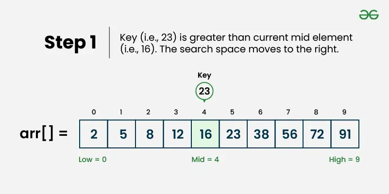 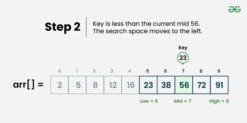 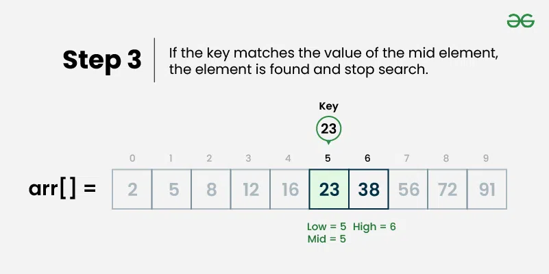 ## Use Cases [Section titled “Use Cases”](#use-cases) * **Large sorted datasets:** When you have large amounts of sorted data * **Database indexing:** Used in database systems for fast record retrieval * **Dictionary lookups:** Finding words in sorted dictionaries * **Library systems:** Searching books by ISBN or catalog numbers ## Time Complexity [Section titled “Time Complexity”](#time-complexity) * **Best case:** O(1) - Element found at middle position * **Average case:** O(log n) - Element found after several divisions * **Worst case:** O(log n) - Element not found or at the edges ## Space Complexity [Section titled “Space Complexity”](#space-complexity) * **Iterative:** O(1) - Constant space * **Recursive:** O(log n) - Due to recursion stack ## Advantages [Section titled “Advantages”](#advantages) * **Very efficient:** O(log n) time complexity is much faster than O(n) * **Predictable performance:** Logarithmic time even in worst case * **Memory efficient:** Iterative version uses constant space * **Simple concept:** Easy to understand the divide-and-conquer approach ## Disadvantages [Section titled “Disadvantages”](#disadvantages) * **Requires sorted data:** Array must be sorted beforehand * **Not suitable for small datasets:** Overhead might not be worth it for small arrays * **Static data:** Frequent insertions/deletions can make maintaining sorted order expensive ## Example [Section titled “Example”](#example) ```java public class BinarySearch { // Iterative binary search method public static int binarySearch(int[] array, int target) { // 📌 Part 1: Initialize left and right pointers int left = 0; int right = array.length - 1; // 📌 Part 2: Loop until left pointer exceeds right pointer while (left <= right) { // 📌 Part 3: Calculate middle index int middle = left + (right - left) / 2; // 📌 Part 4: Check if target is at middle if (target == array[middle]) { return middle; } // 📌 Part 5: If target is smaller, search left half if (target < array[middle]) { right = middle - 1; } // 📌 Part 6: If target is larger, search right half else { left = middle + 1; } } return -1; // Element not found } public static void main(String[] args) { int[] sortedNumbers = {11, 12, 22, 25, 34, 64, 90}; // Must be sorted! int target = 64; System.out.println("Sorted Array: [11, 12, 22, 25, 34, 64, 90]"); System.out.println("Target: " + target); // Using iterative approach int result = binarySearch(sortedNumbers, target); if (result != -1) { System.out.println("Element found at index: " + result); } else { System.out.println("Element not found"); } } } ``` ### Visualization [Section titled “Visualization”](#visualization)  # Bubble Sort > Understanding bubble sort algorithm Bubble sort is a simple sorting algorithm that repeatedly steps through the list, compares adjacent elements, and swaps them if they are in the wrong order. The process is repeated until the list is sorted. It’s called “bubble” sort because larger elements “bubble” to the top of the list. [Play](https://youtube.com/watch?v=kPRA0W1kECg) ## Properties [Section titled “Properties”](#properties) * **Comparison-based:** Works by comparing adjacent elements * **In-place sorting:** Sorts the array without using extra space * **Stable algorithm:** Maintains relative order of equal elements * **Simple implementation:** Easy to understand and implement ## How it Works [Section titled “How it Works”](#how-it-works) 1. **Start from beginning:** Begin with the first element of the array 2. **Compare adjacent elements:** Compare current element with the next element 3. **Swap if needed:** If current element is greater than next, swap them 4. **Move to next pair:** Continue comparing adjacent pairs through the array 5. **Complete one pass:** After one complete pass, the largest element is in its correct position 6. **Repeat:** Repeat the process for remaining unsorted elements 7. **Optimization:** In each pass, ignore the last sorted elements 8. **Done:** Continue until no swaps are needed 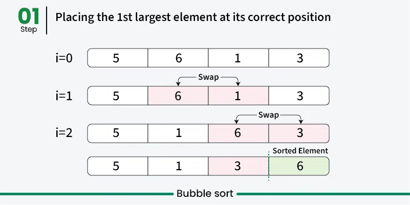 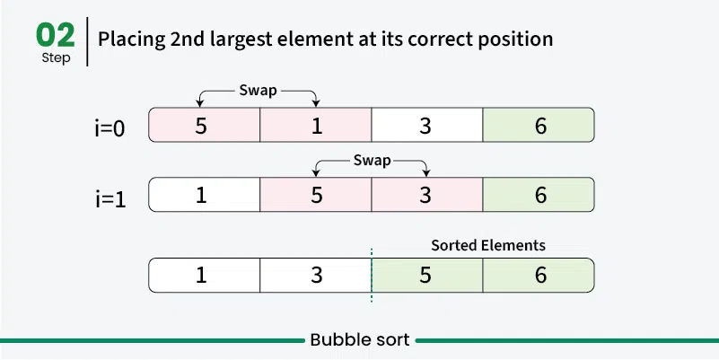 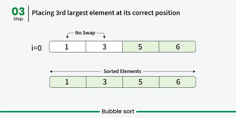 ## Use Cases [Section titled “Use Cases”](#use-cases) * **Educational purposes:** Great for learning sorting concepts * **Small datasets:** Acceptable performance for very small arrays * **Nearly sorted data:** Performs better when data is already mostly sorted * **Simple implementation needed:** When code simplicity is more important than efficiency ## Time Complexity [Section titled “Time Complexity”](#time-complexity) * **Best case:** O(n) - When array is already sorted (with optimization) * **Average case:** O(n²) - Random order of elements * **Worst case:** O(n²) - When array is reverse sorted ## Space Complexity [Section titled “Space Complexity”](#space-complexity) * **O(1):** Constant space, only uses a few variables for swapping ## Advantages [Section titled “Advantages”](#advantages) * **Simple to understand:** Very intuitive algorithm * **In-place sorting:** Doesn’t require additional memory * **Stable:** Maintains relative order of equal elements * **Adaptive:** Can be optimized to detect if array is already sorted ## Disadvantages [Section titled “Disadvantages”](#disadvantages) * **Poor performance:** O(n²) time complexity makes it inefficient for large datasets * **Too many comparisons:** Even for small improvements, requires many comparisons * **Not practical:** Rarely used in real-world applications due to poor performance ## Example [Section titled “Example”](#example) ```java public class BubbleSort { // Bubble sort (stops early if array becomes sorted) public static void bubbleSort(int[] array) { boolean swapped; // 📌 Part 1: Outer loop for number of passes for (int i = 0; i < array.length - 1; i++) { swapped = false; // 📌 Part 2: Inner loop for comparing adjacent elements // Reduce the range in each pass since largest elements bubble up for (int j = 0; j < array.length - i - 1; j++) { // 📌 Part 3: Compare adjacent elements if (array[j] > array[j + 1]) { // 📌 Part 4: Swap elements int temp = array[j]; array[j] = array[j + 1]; array[j + 1] = temp; // Mark that a swap occurred swapped = true; } } // If no swapping occurred, array is sorted if (!swapped) { break; } } } public static void main(String[] args) { int[] numbers = {64, 34, 25, 12, 22, 11, 90}; System.out.print("Original: "); for (int num : numbers) { System.out.print(num + " "); } bubbleSort(numbers); System.out.println(); System.out.print("Sorted: "); for (int num : numbers) { System.out.print(num + " "); } } } ``` ### Visualization [Section titled “Visualization”](#visualization)  # Insertion Sort > Understanding insertion sort algorithm Insertion sort is a simple sorting algorithm that builds the final sorted array one element at a time. It works by taking elements from the unsorted portion and inserting them into their correct position in the sorted portion, similar to how you might sort playing cards in your hand. [Play](https://youtube.com/watch?v=kPRA0W1kECg) ## Properties [Section titled “Properties”](#properties) * **Comparison-based:** Works by comparing elements to find correct position * **In-place sorting:** Sorts the array without using extra space * **Stable algorithm:** Maintains relative order of equal elements * **Adaptive:** Performs better on partially sorted arrays ## How it Works [Section titled “How it Works”](#how-it-works) 1. **Start with second element:** Assume first element is already “sorted” 2. **Pick current element:** Take the next element from unsorted portion 3. **Compare with sorted elements:** Compare with elements in sorted portion (from right to left) 4. **Shift elements:** Move larger elements one position to the right 5. **Insert in correct position:** Place current element in its correct position 6. **Expand sorted portion:** The sorted portion now includes the inserted element 7. **Repeat:** Continue with next element until all elements are processed 8. **Done:** Array is fully sorted 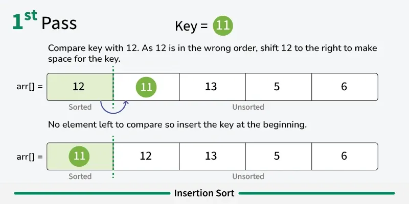 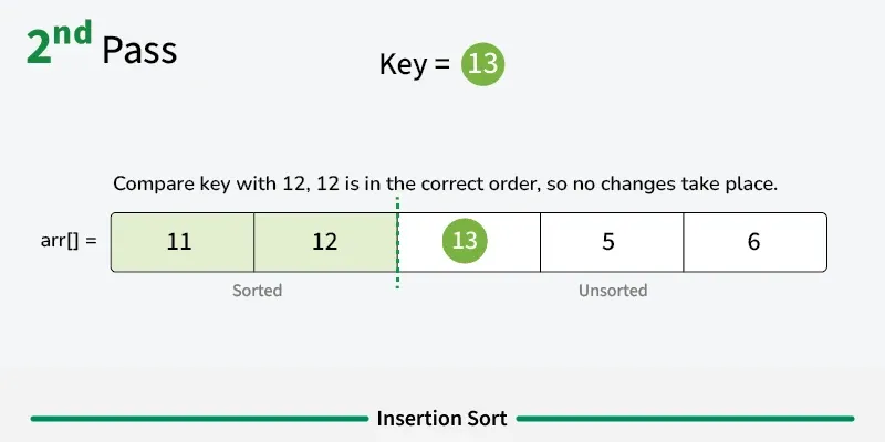 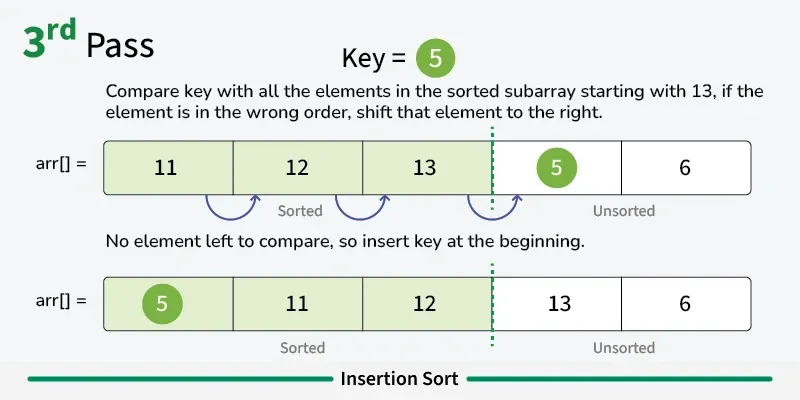 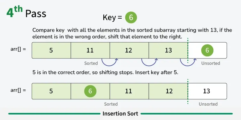 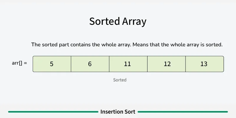 ## Use Cases [Section titled “Use Cases”](#use-cases) * **Small datasets:** Efficient for small arrays (typically < 50 elements) * **Nearly sorted data:** Performs excellently on already sorted or nearly sorted data * **Online algorithm:** Can sort data as it’s received * **Hybrid sorting algorithms:** Used as a subroutine in advanced algorithms like Quicksort ## Time Complexity [Section titled “Time Complexity”](#time-complexity) * **Best case:** O(n) - When array is already sorted * **Average case:** O(n²) - Random order of elements * **Worst case:** O(n²) - When array is reverse sorted ## Space Complexity [Section titled “Space Complexity”](#space-complexity) * **O(1):** Constant space, only uses a few variables ## Advantages [Section titled “Advantages”](#advantages) * **Simple implementation:** Easy to understand and code * **Efficient for small datasets:** Better than other O(n²) algorithms for small arrays * **Adaptive:** Performance improves with partially sorted data * **Stable:** Maintains relative order of equal elements * **In-place:** Requires only constant extra memory * **Online:** Can process elements as they arrive ## Disadvantages [Section titled “Disadvantages”](#disadvantages) * **Poor performance on large datasets:** O(n²) time complexity is inefficient for large arrays * **More comparisons than selection sort:** Generally performs more comparisons * **Not suitable for large-scale applications:** Better algorithms exist for large datasets ## Example [Section titled “Example”](#example) ```java public class InsertionSort { // Basic insertion sort implementation public static void insertionSort(int[] array) { // 📌 Part 1: Start from second element (index 1) since first element is considered sorted for (int i = 1; i < array.length; i++) { // 📌 Part 2: Keep track of current element and last sorted position int currentElement = array[i]; // Element to be inserted int j = i - 1; // Index of last element in sorted portion // 📌 Part 3: Shift elements that are greater than currentElement to one position ahead while (j >= 0 && array[j] > currentElement) { array[j + 1] = array[j]; // Shift element to right j--; } // 📌 Part 4: Insert currentElement at its correct position array[j + 1] = currentElement; } } public static void main(String[] args) { int[] numbers = {64, 34, 25, 12, 22, 11, 90}; System.out.print("Original: "); for (int num : numbers) { System.out.print(num + " "); } insertionSort(numbers); System.out.println(); System.out.print("Sorted: "); for (int num : numbers) { System.out.print(num + " "); } } } ``` ### Visualization [Section titled “Visualization”](#visualization)  # Linear Search > Understanding linear search algorithm Linear search is the simplest searching algorithm that sequentially checks each element in a list until the target element is found or the entire list has been searched. ## Properties [Section titled “Properties”](#properties) * **Sequential access:** Examines elements one by one from the beginning * **Works on any data structure:** Can be used on arrays, linked lists, etc. * **No sorting requirement:** Works on both sorted and unsorted data * **Simple implementation:** Easy to understand and implement ## How it Works [Section titled “How it Works”](#how-it-works) 1. **Start at the beginning:** Begin with the first element of the array 2. **Compare:** Check if the current element matches the target value 3. **Found:** If match found, return the index/position 4. **Move to next:** If no match, move to the next element 5. **Repeat:** Continue until element is found or end of array is reached 6. **Not found:** If end is reached without finding the element, return -1 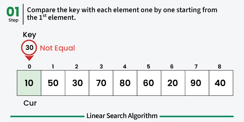 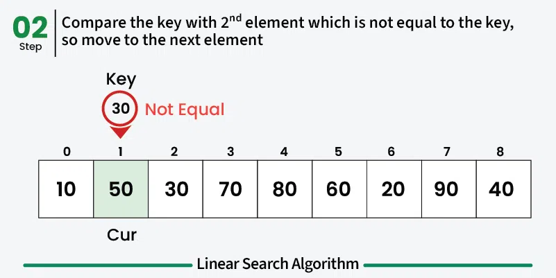 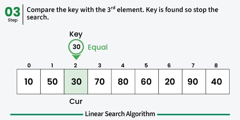 ## Use Cases [Section titled “Use Cases”](#use-cases) * **Small datasets:** When the dataset is small and simplicity is preferred * **Unsorted data:** When data is not sorted and sorting would be expensive * **One-time search:** When searching is done infrequently * **Memory-constrained environments:** When memory usage needs to be minimal ## Time Complexity [Section titled “Time Complexity”](#time-complexity) * **Best case:** O(1) - Element found at first position * **Average case:** O(n) - Element found in the middle * **Worst case:** O(n) - Element not found or at the last position ## Space Complexity [Section titled “Space Complexity”](#space-complexity) * **O(1):** Constant space, only uses a few variables ## Advantages [Section titled “Advantages”](#advantages) * **Simple to implement:** Easy to understand and code * **No preprocessing required:** Works directly on unsorted data * **Memory efficient:** Uses constant extra space * **Works on any data structure:** Can be applied to arrays, linked lists, etc. ## Disadvantages [Section titled “Disadvantages”](#disadvantages) * **Slow for large datasets:** O(n) time complexity makes it inefficient for large data * **Not optimal:** Other algorithms like binary search are much faster for sorted data ## Example [Section titled “Example”](#example) ```java public class LinearSearch { // Method to perform linear search public static int linearSearch(int[] array, int target) { // 📌 Part 1: Iterate through each element in the array for (int i = 0; i < array.length; i++) { // 📌 Part 2: Check if current element matches the target if (array[i] == target) { return i; // Return the index if found } } return -1; // Return -1 if element not found } public static void main(String[] args) { int[] numbers = {64, 34, 25, 12, 22, 11, 90}; int target = 22; System.out.println("Array: [64, 34, 25, 12, 22, 11, 90]"); System.out.println("Target: " + target); int result = linearSearch(numbers, target); if (result != -1) { System.out.println("Element found at index: " + result); } else { System.out.println("Element not found in the array"); } } } ``` ### Visualization [Section titled “Visualization”](#visualization)  # Selection Sort > Understanding selection sort algorithm Selection sort is a simple sorting algorithm that works by repeatedly finding the minimum element from the unsorted portion and placing it at the beginning. It divides the array into a sorted portion (initially empty) and an unsorted portion (initially the entire array). [Play](https://youtube.com/watch?v=kPRA0W1kECg) ## Properties [Section titled “Properties”](#properties) * **Comparison-based:** Works by comparing elements to find minimum * **In-place sorting:** Sorts the array without using extra space * **Unstable algorithm:** Does not maintain relative order of equal elements * **Simple implementation:** Easy to understand and implement ## How it Works [Section titled “How it Works”](#how-it-works) 1. **Start with first position:** Assume first element is the minimum 2. **Find minimum in unsorted portion:** Scan through unsorted part to find the actual minimum 3. **Swap with first position:** Replace the first element with the found minimum 4. **Move to next position:** The first element is now sorted, move to second position 5. **Repeat:** Find minimum in remaining unsorted portion and swap with current position 6. **Continue:** Repeat until all elements are in their correct positions 7. **Done:** Array is fully sorted when all positions are filled    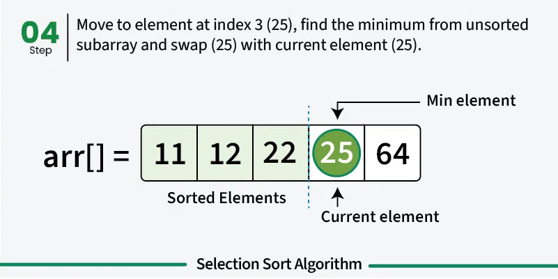 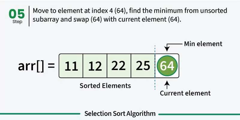 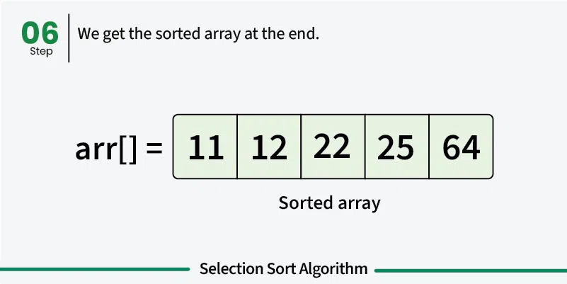 ## Use Cases [Section titled “Use Cases”](#use-cases) * **Educational purposes:** Good for learning sorting concepts * **Small datasets:** Acceptable for very small arrays * **Memory-constrained environments:** Uses minimal extra memory * **When simplicity matters:** When implementation simplicity is priority ## Time Complexity [Section titled “Time Complexity”](#time-complexity) * **Best case:** O(n²) - Even when array is already sorted * **Average case:** O(n²) - Random order of elements * **Worst case:** O(n²) - When array is reverse sorted **Note:** Unlike bubble sort, selection sort always performs O(n²) comparisons regardless of input. ## Space Complexity [Section titled “Space Complexity”](#space-complexity) * **O(1):** Constant space, only uses a few variables ## Advantages [Section titled “Advantages”](#advantages) * **Simple to understand:** Intuitive algorithm concept * **In-place sorting:** Minimal memory requirements * **Consistent performance:** Always O(n²), predictable behavior * **Minimum number of swaps:** Makes at most n-1 swaps ## Disadvantages [Section titled “Disadvantages”](#disadvantages) * **Poor performance:** O(n²) time complexity for all cases * **Not adaptive:** Doesn’t improve performance for partially sorted arrays * **Unstable:** May change relative order of equal elements * **Not suitable for large datasets:** Inefficient for large arrays ## Example [Section titled “Example”](#example) ```java public class SelectionSort { // Selection sort implementation public static void selectionSort(int[] array) { // 📌 Part 1: Traverse through all array elements for (int i = 0; i < array.length - 1; i++) { // 📌 Part 2: Find the minimum element in remaining unsorted array int minIndex = i; // 📌 Part 3: Scan through unsorted portion for (int j = i + 1; j < array.length; j++) { // 📌 Part 4: Update minIndex if current element is smaller if (array[j] < array[minIndex]) { minIndex = j; } } // 📌 Part 5: Swap the found minimum element with the first element if (minIndex != i) { int temp = array[minIndex]; array[minIndex] = array[i]; array[i] = temp; } } } public static void main(String[] args) { int[] numbers = {64, 34, 25, 12, 22, 11, 90}; System.out.print("Original: "); for (int num : numbers) { System.out.print(num + " "); } selectionSort(numbers); System.out.println(); System.out.print("Sorted: "); for (int num : numbers) { System.out.print(num + " "); } } } ``` ### Visualization [Section titled “Visualization”](#visualization)  # Time & Space Complexity > Understanding time and space complexity analysis Big O notation is used to describe both time complexity and space complexity: * **Time complexity** (using Big O) tells us how the running time of an algorithm increases as the input gets bigger. * **Space complexity** (using Big O) tells us how the memory usage of an algorithm increases as the input gets bigger. ## Time Complexity [Section titled “Time Complexity”](#time-complexity) Time complexity tells us how long an algorithm takes to run as the input gets bigger. It helps us understand if our code will still be fast when working with large amounts of data. * Lower time complexity means faster code for big inputs. ### Why is it important? [Section titled “Why is it important?”](#why-is-it-important) * It helps you pick the best algorithm for the job. * It shows how your code will scale as data grows. ### Example [Section titled “Example”](#example) * If you loop through a list of 10 items, it takes about 10 steps. If the list has 1,000 items, it takes about 1,000 steps. This is **O(n)** time. * If you always do the same number of steps, no matter how big the input is, that’s **O(1)** time. ## Space Complexity [Section titled “Space Complexity”](#space-complexity) ### What is Space Complexity? [Section titled “What is Space Complexity?”](#what-is-space-complexity) Space complexity tells us how much extra memory (RAM) an algorithm needs as the input gets bigger. This includes variables, data structures, and function call stacks. * Lower space complexity means your code uses less memory and can handle bigger problems. ### Why is it important? [Section titled “Why is it important?”](#why-is-it-important-1) * It helps you avoid running out of memory. * It shows if your code is efficient with resources. ### Example [Section titled “Example”](#example-1) * If you only use a few variables, no matter how big the input is, that’s **O(1)** space. * If you make a new list as big as the input, that’s **O(n)** space. # Data Structures > Fundamental concepts of data structures Data Structures are a way of collecting and organising data in such a way that we can perform operations on these data in an effective way. ## Types of Data Structures [Section titled “Types of Data Structures”](#types-of-data-structures)  * [**Primitive**](#primitive-data-structures): Integer, Character, Boolean, Float, etc. * [**Non-Primitive**](#non-primitive-data-structures): * **Linear**: * Arrays * Lists * Linked Lists * Stacks * Queues * **Non-Linear**: ❌ * Trees * HashMaps * Graphs ## Primitive Data Structures [Section titled “Primitive Data Structures”](#primitive-data-structures) These are basic built-in data types in Java. | Type | Description | Example | | --------- | ------------------------------------------------------ | ---------------------- | | `int` | 32-bit integer, range: -2,147,483,648 to 2,147,483,647 | `int i = 123456;` | | `char` | Single 16-bit Unicode character | `char c = 'A';` | | `boolean` | True or false value | `boolean flag = true;` | | `float` | 32-bit floating-point, single precision | `float f = 3.14f;` | | `double` | 64-bit floating-point, double precision | `double d = 3.14159;` | | `byte` | 8-bit integer, range: -128 to 127 | `byte b = 100;` | | `short` | 16-bit integer, range: -32,768 to 32,767 | `short s = 20000;` | | `long` | 64-bit integer, range: very large whole numbers | `long l = 123456789L;` | ## Non-Primitive Data Structures [Section titled “Non-Primitive Data Structures”](#non-primitive-data-structures) Are more complex and are made up of primitive data types. They can be divided into two types: * Linear Data Structures * Non-linear Data Structures ### Linear Data Structures [Section titled “Linear Data Structures”](#linear-data-structures) Data elements are arranged in a sequential manner, where each element is connected to its previous and next element. * [Arrays](/algos-ds/data-structures/arrays) * [Lists](/algos-ds/data-structures/lists) * [Linked Lists](/algos-ds/data-structures/linked-lists) * [Stacks](/algos-ds/data-structures/stacks) * [Queues](/algos-ds/data-structures/queues) ### Non-Linear Data Structures [Section titled “Non-Linear Data Structures”](#non-linear-data-structures) Data elements are not arranged sequentially - they can have multiple connections. * [Trees](/algos-ds/data-structures/trees) * [HashMaps](/algos-ds/data-structures/hashmaps) * [Graphs](/algos-ds/data-structures/graphs) # Arrays > Understanding arrays data structure 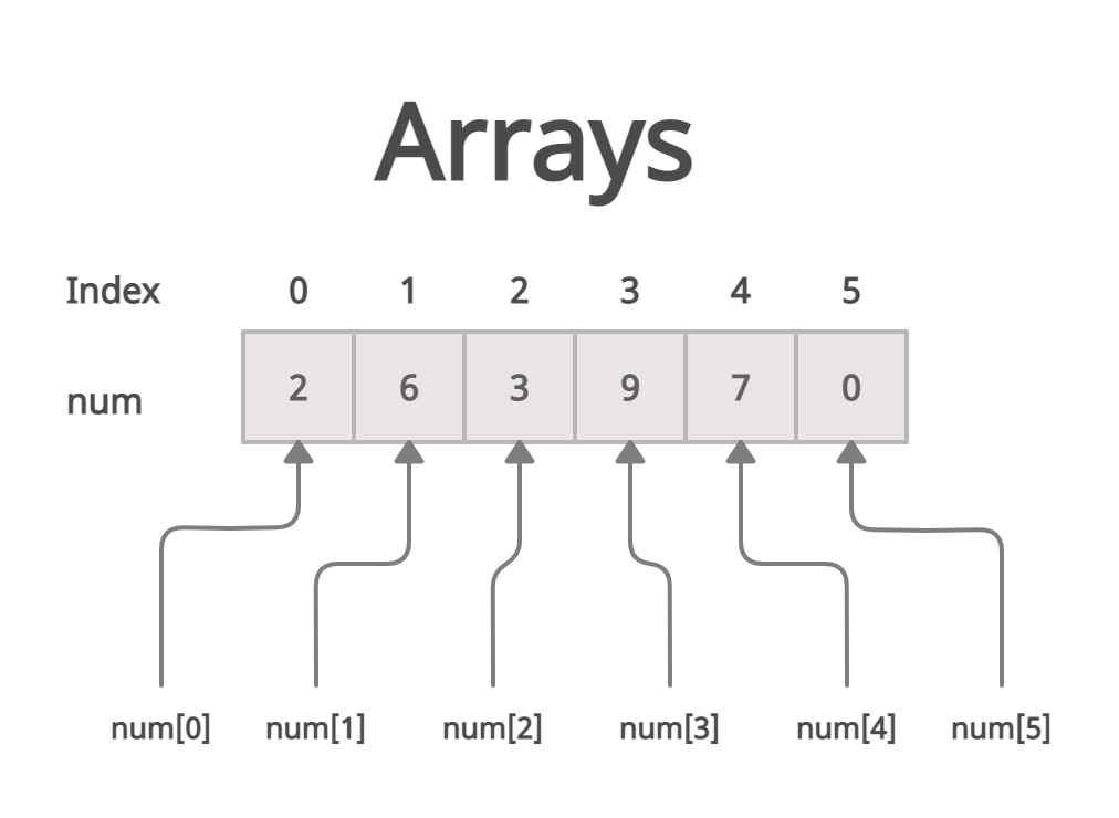 Fixed-size collection of elements of the same type, stored in contiguous memory locations. ### Properties [Section titled “Properties”](#properties) * **Fixed size:** Size is set when created and cannot change. * **Contiguous memory:** Elements are stored next to each other. * **Random access:** Any element can be accessed directly by index. * **Same type:** All elements must be of the same data type. * **Allows duplicates:** Repeated values are permitted. ### Operations [Section titled “Operations”](#operations) * **Access:** Direct access using index. * **Insertion:** Need to shift elements. * **Update:** Directly modify an element by index. * **Deletion:** Need to shift elements after deletion. ### Advantages [Section titled “Advantages”](#advantages) * **Fast access:** Elements can be quickly accessed using their index. * **Memory efficient:** Elements are stored together in memory, reducing overhead. ### Disadvantages [Section titled “Disadvantages”](#disadvantages) * **Fixed size:** Cannot be resized after creation. * **Manual insertion and deletion:** Adding or removing elements requires shifting other elements. * **Memory waste:** Unused space is wasted if the array is not fully filled. ### Example [Section titled “Example”](#example) ```java // Declaration and initialization int[] numbers = {1, 2, 3, 4, 5}; // Declare and set the size of the array String[] students = new String[3]; // Insert elements students[0] = "Dustin"; students[1] = "Rewish"; students[2] = "Ada Lovelace"; // Accessing an element System.out.println(students[0]); // Prints "Dustin" // Updating an element students[0] = "Dustin VII"; // Updates "Dustin" to "Dustin VII" System.out.println(students[0]); // Deleting an element students[2] = null; // Removes "Ada Lovelace" System.out.println(students[2]); // Prints "null" ``` # Graphs > Understanding graphs data structure 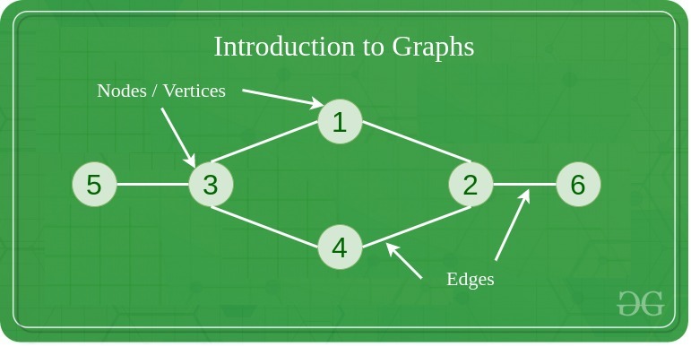 A graph is a non-linear data structure consisting of vertices (nodes) connected by edges (links). Unlike trees, graphs can have cycles and multiple paths between nodes. Think of it like a network of cities connected by roads, where you can travel between cities through various routes. ### Properties [Section titled “Properties”](#properties) * **Set of vertices (nodes) and edges (connections):** The fundamental components that make up a graph structure. * **Can be directed or undirected:** Edges may have direction (one-way) or be bidirectional (two-way). * **Can be weighted or unweighted:** Edges may have associated costs or values, or all be considered equal. * **Can be cyclic or acyclic:** May contain loops that return to the starting vertex or be cycle-free. * **Can be connected or disconnected:** All vertices may be reachable from each other, or exist in separate components. ### Use Cases [Section titled “Use Cases”](#use-cases) * **Social networks:** Representing relationships between people (friends, followers, connections). * **Transportation networks:** Modeling roads, flight routes, and public transit systems. * **Computer networks:** Representing connections between computers, routers, and servers. * **Dependency graphs:** Showing dependencies between tasks, modules, or packages. * **Game maps and pathfinding:** Creating navigable game worlds and finding optimal routes. * **Web page linking:** Representing hyperlinks between web pages for search engines. ### Types [Section titled “Types”](#types) * Directed Graph: Edges have direction * Undirected Graph: Edges have no direction * Weighted Graph: Edges have weights/costs * Unweighted Graph: All edges have same weight * Complete Graph: Every vertex connected to every other vertex * Bipartite Graph: Vertices can be divided into two disjoint sets ### Representations [Section titled “Representations”](#representations) * Adjacency Matrix: 2D array of connections * Adjacency List: List of neighbors for each vertex * Edge List: List of all edges ### Operations [Section titled “Operations”](#operations) * **Add Vertex:** O(1) in adjacency list - Add a new node to the graph. * **Add Edge:** O(1) in adjacency list - Create a connection between two vertices. * **Remove Vertex:** O(V + E) where V = vertices, E = edges - Delete a node and all its connections. * **Remove Edge:** O(V) in adjacency list - Remove a connection between two vertices. * **Find Edge:** O(V) in adjacency list, O(1) in adjacency matrix - Check if two vertices are connected. ### Traversal Algorithms [Section titled “Traversal Algorithms”](#traversal-algorithms) * Depth-First Search (DFS): Uses stack/recursion * Breadth-First Search (BFS): Uses queue * Both have O(V + E) time complexity ### Advantages [Section titled “Advantages”](#advantages) * **Models complex relationships:** Can represent any type of connection between entities. * **Flexible structure:** Supports various types of connections and relationships. * **Many algorithms available:** Rich set of algorithms for traversal, shortest path, and analysis. * **Real-world problem modeling:** Natural representation for many practical problems. * **Powerful analysis capabilities:** Can analyze connectivity, centrality, and network properties. ### Disadvantages [Section titled “Disadvantages”](#disadvantages) * **Complex implementation:** More complicated to implement compared to linear data structures. * **High memory usage for dense graphs:** Adjacency matrices use O(V²) space regardless of edge count. * **Some operations can be expensive:** Operations like finding shortest paths can be computationally intensive. * **No guaranteed ordering:** Unlike trees, graphs don’t have a natural hierarchical structure. * **Potential for infinite loops:** Cycles in graphs can cause algorithms to run indefinitely without proper handling. ### Example [Section titled “Example”](#example) ```java import java.util.*; // Graph implementation using adjacency list class Graph { private Map> adjacencyList; public Graph() { adjacencyList = new HashMap<>(); } // Add a vertex to the graph public void addVertex(int vertex) { adjacencyList.putIfAbsent(vertex, new ArrayList<>()); } // Add an edge between two vertices (undirected) public void addEdge(int source, int destination) { adjacencyList.get(source).add(destination); adjacencyList.get(destination).add(source); // For undirected graph } // Display the graph public void displayGraph() { for (int vertex : adjacencyList.keySet()) { System.out.println(vertex + " -> " + adjacencyList.get(vertex)); } } } // Usage example Graph graph = new Graph(); // Add vertices graph.addVertex(1); graph.addVertex(2); graph.addVertex(3); graph.addVertex(4); // Add edges (connections) graph.addEdge(1, 2); // Connect 1 to 2 graph.addEdge(1, 3); // Connect 1 to 3 graph.addEdge(2, 4); // Connect 2 to 4 graph.addEdge(3, 4); // Connect 3 to 4 // Display the graph graph.displayGraph(); // Output: // 1 -> [2, 3] // 2 -> [1, 4] // 3 -> [1, 4] // 4 -> [2, 3] ``` # HashMaps > Understanding hashmaps data structure 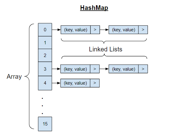 A HashMap is a data structure that stores key-value pairs and uses a hash function to compute an index for fast data retrieval. It’s like a digital phone book where you can quickly find someone’s number (value) by looking up their name (key), regardless of how many contacts you have. ### Properties [Section titled “Properties”](#properties) * **Key-value pair storage:** Each element consists of a unique key associated with a value. * **Uses hash function to compute index:** Keys are converted to array indices using mathematical functions. * **Keys must be unique:** No duplicate keys are allowed, but values can be duplicated. ### Use Cases [Section titled “Use Cases”](#use-cases) * **Caching systems:** Storing frequently accessed data for quick retrieval. ### Operations [Section titled “Operations”](#operations) * **Search:** Find a value using its key. * **Insertion:** Add a new key-value pair. * **Deletion:** Remove a key-value pair. * **Access:** Retrieve a value using its key. * **Update:** Modify the value associated with a key. ### Advantages [Section titled “Advantages”](#advantages) * **Very fast average-case operations:** Most operations complete in constant time on average. * **Flexible key types:** Can use various data types as keys (strings, numbers, objects). * **Dynamic sizing:** Can grow and shrink as needed during runtime. ### Disadvantages [Section titled “Disadvantages”](#disadvantages) * **No ordering of elements:** Elements are not stored in any predictable sequence. ### Example [Section titled “Example”](#example) ```java import java.util.HashMap; HashMap studentGrades = new HashMap<>(); // Insert key-value pairs studentGrades.put("Swasti", 95); studentGrades.put("Terrence", 87); studentGrades.put("Shafeer", 82); // Access values using keys System.out.println(studentGrades.get("Swasti")); // Prints 95 // Update existing value studentGrades.put("Swasti", 100); System.out.println(studentGrades.get("Swasti")); // Prints 100 // Get size of the map System.out.println(studentGrades.size()); // Prints 3 // Remove a key-value pair studentGrades.remove("Shafeer"); System.out.println(studentGrades); // Iterate through the map for (String student : studentGrades.keySet()) { System.out.println(student + ": " + studentGrades.get(student)); } ``` # Linked Lists > Understanding linked lists data structure 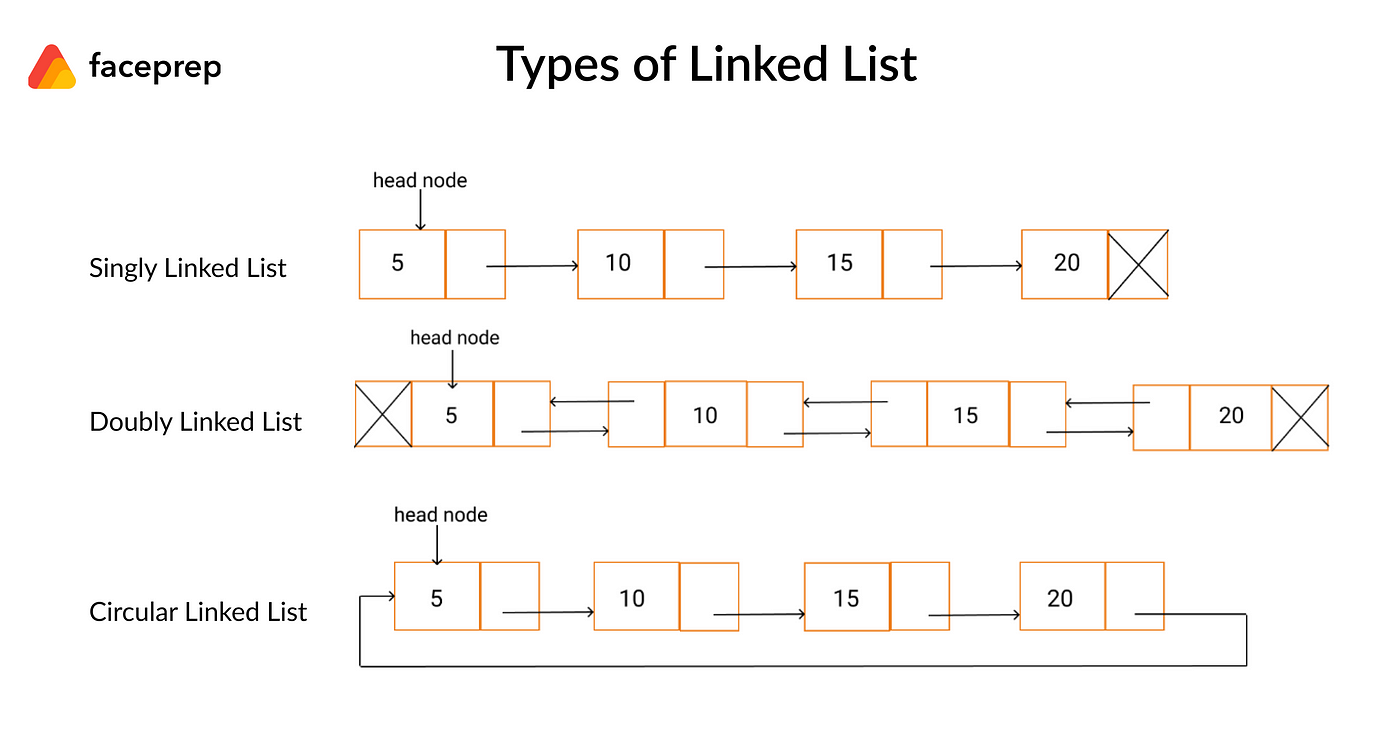 Collection of nodes where each node contains data and a reference to the next node. ### Types [Section titled “Types”](#types) * **Singly Linked List**: One pointer to next node. * **Doubly Linked List**: Pointers to both next and previous nodes. * **Circular Linked List**: Last node points back to first node. ### Use Cases [Section titled “Use Cases”](#use-cases) * **Music playlists:** Songs are linked together, allowing easy addition, removal, and reordering. * **Image viewers:** Navigating through images in a gallery uses linked lists for previous/next functionality. ### Properties [Section titled “Properties”](#properties) * **Node structure:** Each node has data and a pointer to the next. * **Dynamic size:** Grows or shrinks as needed. * **Non-contiguous memory:** Nodes are scattered in memory. * **No random access:** Must traverse from the head. * **Types:** Can be singly, doubly, or circular. ### Operations [Section titled “Operations”](#operations) * **Access:** Traverse from the head to find an element. * **Insertion:** Add a new node at a specific position. * **Update:** Change the data in a node. * **Deletion:** Remove a node from a specific position. ### Advantages [Section titled “Advantages”](#advantages) * **Dynamic size:** The list can grow or shrink as needed. * **Memory allocated as needed:** Nodes are created only when required. * **No memory waste:** Only necessary memory is used, no pre-allocation. ### Disadvantages [Section titled “Disadvantages”](#disadvantages) * **No random access:** You cannot directly access an element by index; must traverse from the head. * **Sequential access only:** Elements must be accessed one after another, not directly. * **Extra memory for storing pointers:** Each node needs additional memory for its pointer(s). ### Example [Section titled “Example”](#example) ```java import java.util.LinkedList; import java.util.ListIterator; LinkedList songs = new LinkedList<>(); // Insert nodes songs.add("Kendrick Lamar - Not Like Us"); songs.add("Alex Warren - Ordinary"); songs.add("Drake - Nokia"); // Get number of nodes System.out.println(songs.size()); // Prints 3 // Accessing nodes ListIterator songsIt = songs.listIterator(); while (songsIt.hasNext()) { String song = songsIt.next(); System.out.println(song); } // Updating a node ListIterator songsIt2 = songs.listIterator(); while (songsIt2.hasNext()) { String song = songsIt2.next(); if (song == "Kendrick Lamar - Not Like Us") { songsIt2.set("Kendrick Lamar - Luther"); } } System.out.println(songs); // Deleting a node ListIterator songsIt3 = songs.listIterator(); while (songsIt3.hasNext()) { String song = songsIt3.next(); if (song == "Drake - Nokia") { songsIt3.remove(); } } System.out.println(songs); ``` # Lists > Understanding lists data structure 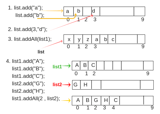 Dynamic arrays that can grow or shrink in size. More flexible than regular arrays. ### Properties [Section titled “Properties”](#properties) * **Dynamic size:** Can grow or shrink during runtime. * **Maintains order:** Elements stay in the order added. * **Allows duplicates:** Repeated values are permitted. ### Operations [Section titled “Operations”](#operations) * **Access:** Directly get an element by its index. * **Insertion:** Add an element at the end or at a specific position. * **Update:** Change the value of an element at a given index. * **Deletion:** Remove an element from the end or from a specific position. ### Advantages [Section titled “Advantages”](#advantages) * **Dynamic sizing:** List can grow or shrink as needed. * **Automatic insertion and deletion:** Adding or removing elements will shift other elements. ### Disadvantages [Section titled “Disadvantages”](#disadvantages) * **More memory overhead:** Lists use extra memory compared to arrays because they store additional information (like capacity, size, and references for dynamic resizing) to support flexible operations. ### Example [Section titled “Example”](#example) ```java import java.util.ArrayList; // List of strings ArrayList students = new ArrayList<>(); // Insert elements students.add("Sher"); students.add("Riaaz"); students.add("Rishika"); students.add("Sem"); // Get number of elements System.out.println(students.size()); // Prints 4 // Accessing an element System.out.println(students.get(0)); // Prints "Sher" // Updating an element students.set(0, "Sherreskly"); // Updates "Sher" to "Sherreskly" System.out.println(students.get(0)); // Deleting an element students.remove(1); // Removes "Riaaz" System.out.println(students.get(1)); // Prints "Rishika" ``` # Queues > Understanding queues data structure 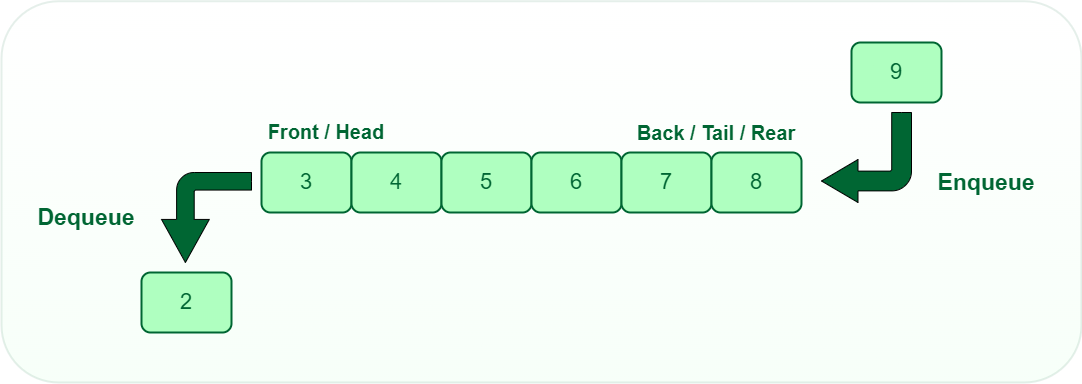 A queue is a linear data structure that follows the First-In-First-Out (FIFO) principle, meaning the first element added is the first one to be removed. Think of it like a line of people waiting - the person who arrives first gets served first. ### Properties [Section titled “Properties”](#properties) * **FIFO (First In, First Out) ordering:** The first element added is the first one to be removed. * **Elements added at rear (enqueue):** New elements are always added to the back of the queue. * **Elements removed from front (dequeue):** Elements are always removed from the front of the queue. * **Can be implemented using arrays or linked lists:** Flexible implementation options depending on needs. ### Use Cases [Section titled “Use Cases”](#use-cases) * **Print job management:** Handling print requests in the order they were submitted. * **Call center systems:** Managing incoming calls in the order they arrive. ### Operations [Section titled “Operations”](#operations) * **Enqueue:** Add element to the rear (back) of the queue. * **Dequeue:** Remove and return element from the front of the queue. ### Advantages [Section titled “Advantages”](#advantages) * **Fair processing (first come, first served):** Ensures elements are processed in the order they arrive. * **Efficient for sequential processing:** All basic operations have O(1) time complexity. * **Easy to implement:** Simple structure with clear insertion and deletion points. ### Disadvantages [Section titled “Disadvantages”](#disadvantages) * **Limited access pattern:** Can only access the front element directly. ### Example [Section titled “Example”](#example) ```java import java.util.Queue; import java.util.LinkedList; Queue students = new LinkedList<>(); // Enqueue elements students.offer("Jalen"); students.offer("Nawiesh"); students.offer("Rafael"); // Get queue size System.out.println(students.size()); // Prints 3 // Accessing the front element System.out.println(students.peek()); // Prints "Jalen" // Dequeue elements students.poll(); // Removes "Jalen", queue: [Nawiesh, Rafael] students.poll(); // Removes "Nawiesh", queue: [Rafael] System.out.println(students); ``` # Stacks > Understanding stacks data structure 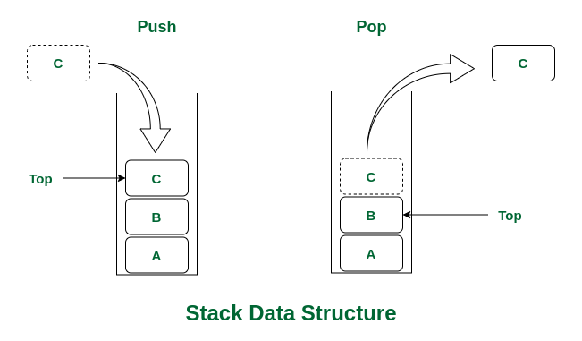 A stack is a linear data structure that follows the Last-In-First-Out (LIFO) principle, meaning the last element added is the first one to be removed. Think of it like a stack of plates - you can only add or remove plates from the top of the stack. ### Properties [Section titled “Properties”](#properties) * **LIFO (Last In, First Out) ordering:** The most recently added element is the first one to be removed. * **Access only to top element:** You can only interact with the element at the top of the stack. * **Limited access pattern:** No random access to elements in the middle of the stack. * **Dynamic size:** Can grow and shrink as elements are added or removed. ### Use Cases [Section titled “Use Cases”](#use-cases) * **Undo operations:** Stacks are used to keep track of previous states, allowing you to undo actions in applications. * **Browser back button:** Web browsers use stacks to remember the sequence of pages visited, enabling you to go back to previous pages. ### Operations [Section titled “Operations”](#operations) * **Push:** Add element to the top of the stack. * **Pop:** Remove and return the top element from the stack. ### Advantages [Section titled “Advantages”](#advantages) * **Simple and efficient operations:** All basic operations have O(1) time complexity. * **Easy to implement:** Simple structure makes implementation straightforward. ### Disadvantages [Section titled “Disadvantages”](#disadvantages) * **Limited access:** Only the top element can be accessed directly, no random access to elements. * **Can overflow:** If size limit exceeded (in array-based implementations), stack overflow can occur. ### Example [Section titled “Example”](#example) ```java import java.util.Stack; Stack students = new Stack<>(); // Push elements onto the stack students.push("Ashitosh"); students.push("Eleanor"); students.push("Othniel"); // Get stack size System.out.println(students.size()); // Prints 3 // Accessing the top element System.out.println(students.peek()); // Prints "Othniel" // Pop elements from the stack students.pop(); // Removes "Othniel", stack: [Ashitosh, Eleanor] students.pop(); // Removes "Eleanor", stack: [Ashitosh] System.out.println(students); ``` # Trees > Understanding trees data structure 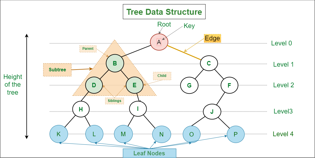 A tree is a hierarchical data structure consisting of nodes connected by edges. It resembles an upside-down tree with a root at the top and branches extending downward. Each node can have multiple children, but only one parent (except the root node which has no parent). ### Properties [Section titled “Properties”](#properties) * **Hierarchical structure with parent-child relationships:** Nodes are organized in levels with clear parent-child connections. * **One root node (no parent):** The top-most node that serves as the starting point of the tree. * **Each node can have multiple children:** Nodes can branch out to any number of child nodes. * **N nodes have N-1 edges:** A tree with N nodes always has exactly N-1 connecting edges. ### Use Cases [Section titled “Use Cases”](#use-cases) * **File systems:** Representing folder and file hierarchies in operating systems. ### Types [Section titled “Types”](#types) * **Binary Tree**: Each node has at most 2 children ### Operations [Section titled “Operations”](#operations) * **Search:** Find a specific value in the tree. * **Insertion:** Add a new node to the tree. * **Deletion:** Remove a node from the tree. * **Traversal:** Visit all nodes in a specific order (Inorder, Preorder, Postorder). ### Traversal Methods [Section titled “Traversal Methods”](#traversal-methods) * **Inorder:** Left → Root → Right * **Preorder:** Root → Left → Right * **Postorder:** Left → Right → Root * **Level order:** Breadth-first traversal ### Advantages [Section titled “Advantages”](#advantages) * **Efficient searching and sorting:** Balanced trees provide logarithmic time complexity for common operations. * **Hierarchical data representation:** Natural way to represent data with parent-child relationships. * **Dynamic size:** Can grow and shrink as needed during runtime. * **Various traversal methods:** Multiple ways to visit and process nodes. ### Disadvantages [Section titled “Disadvantages”](#disadvantages) * **No constant time operations:** Most operations require traversing the tree structure. * **Complex implementation:** More complex to implement compared to linear data structures. * **Recursive nature:** Many tree algorithms are recursive, which can cause stack overflow for very deep trees. ### Example [Section titled “Example”](#example) ```java // Simple binary tree node class class TreeNode { int data; TreeNode left; TreeNode right; TreeNode(int value) { this.data = value; this.left = null; this.right = null; } } // Creating a binary tree TreeNode root = new TreeNode(1); // Root node root.left = new TreeNode(2); // Left child of root root.right = new TreeNode(3); // Right child of root root.left.left = new TreeNode(4); // Left child of node 2 root.left.right = new TreeNode(5); // Right child of node 2 // Tree structure: // 1 // / \ // 2 3 // / \ // 4 5 // Inorder traversal (Left -> Root -> Right) public void inorderTraversal(TreeNode node) { if (node != null) { inorderTraversal(node.left); // Visit left subtree System.out.print(node.data + " "); // Visit root inorderTraversal(node.right); // Visit right subtree } } // Usage: inorderTraversal(root); // Output: 4 2 5 1 3 ``` # Algorithms & Data Structures > Introduction to Algorithms and Data Structures Welcome to the Algorithms & Data Structures subject. This subject covers fundamental concepts of algorithmic thinking, data organization, and computational problem-solving. ## Subject Overview [Section titled “Subject Overview”](#subject-overview) This subject is structured into sections: ### Data Structures [Section titled “Data Structures”](#data-structures) * [Introduction](/algos-ds/data-structures) * [Arrays](/algos-ds/data-structures/arrays) * [Lists](/algos-ds/data-structures/lists) * [Linked Lists](/algos-ds/data-structures/linked-lists) * [Stacks](/algos-ds/data-structures/stacks) * [Queues](/algos-ds/data-structures/queues) * [Trees](/algos-ds/data-structures/trees) * [HashMaps](/algos-ds/data-structures/hashmaps) * [Graphs](/algos-ds/data-structures/graphs) ### Algorithms [Section titled “Algorithms”](#algorithms) * [Introduction](/algos-ds/algorithms) * [Big O Notation](/algos-ds/algorithms/big-o-notation) * [Time & Space Complexity](/algos-ds/algorithms/time-space-complexity) ### Searching Algorithms [Section titled “Searching Algorithms”](#searching-algorithms) * [Linear Search](/algos-ds/algorithms/linear-search) * [Binary Search](/algos-ds/algorithms/binary-search) ### Sorting Algorithms [Section titled “Sorting Algorithms”](#sorting-algorithms) * [Bubble Sort](/algos-ds/algorithms/bubble-sort) * [Selection Sort](/algos-ds/algorithms/selection-sort) * [Insertion Sort](/algos-ds/algorithms/insertion-sort)